Tools and techniques for strategic analysis: The experience curve

The phrase experience curve is small concept and used many decades ago to define the mathematical relation between the cumulated output of a product and its costs. It was invented in Boston consultancy group in 1968. The work was initially for analysing numerous chemical and electronic industries in the decade of sixties. Work was used to explain the price and competitive behaviour of fast growing market segment in these industries (Drejer, 2002). All cost and effects are mirrored by experience curve. The experience curve used extensively after the mid-1960s when it was proved to be an influential analytical tool for the increasing chemical and electronics industries. Several studies have shown that production costs usually decline by 10% to 30% with each doubling of cumulated output.

According to Bhalla, three main factors are responsible for existence of experience curve that include learning, economies of scale and technology (1987).

The experience curve proposes that the company with the highest share of an industry's cumulated output will also be the low-cost producer. Some consulting firms have contended that a business unit's route to a cost advantage lies through cutting price in order to buy share. The increased share of current output is supposed to push the aggressive business unit's costs down the experience curve more rapidly than its competitors', thus improving its comparative position (Kozami, 2002).

Experience curve strategies generally gain greatest leverage early in a product's life cycle because cumulated output doubles very rapidly at this stage. Policies of experience curve are particularly suitable when a company's product is very sensitive to price changes. Cutting prices in such industries leads to huge jumps in demand. This additional demand quickens the company's development down the experience curve by permitting rapid increases in cumulated output. The lower costs result provide leeway for the next round of price cuts and the process repeats itself.

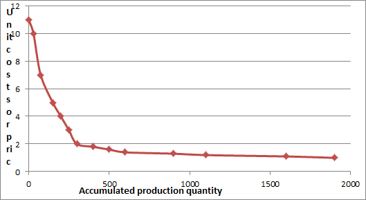
Learning curve can be graphically represented with in coordinate system in which the unit costs are presented on the ordinate and accumulated production quantities are shown on the abscissa (Reichmann, 2012).

Example of experience curve (Source: Reichmann, 2012)

The experience curve is defined by a power law function sometimes referred to as Henderson's Law:
Cn = C1 n-a
Where:
C1 is the cost of the first unit of production
Cn is the cost of the nth unit of production
n is the cumulative volume of production
a is the elasticity of cost with regard to output

Uses of Experience Curve

There are three areas where experience curves are used that include strategic, internal, and external to the organization.
Strategic uses include determining volume-cost changes, estimating new product start-up costs, and pricing of new products.
Internal applications include developing labour standards, scheduling, budgeting, and make-or-buy decisions.
External uses are supplier scheduling, cash flow budgeting, and estimating purchase costs.

Disparagements of the Experience Curve

It has been perceived that experience curve should not be observed in isolation. Experience curve has a strong dependency on individuals under observation. If the outlook of the individual is positive, the resulting curve will resemble learning curve but if the attitude of the individual is negative, the resulting curve will not hold good.

To summarize, experience curve explains the efficiency increase gained by workers through repetitive productive work. Experience curve is based on the commonly observed phenomenon that unit cost decline as a firm accumulate experience in terms of cumulative volume of production.